JAX 中的廣義卷積#
![]()

JAX 提供了許多介面來計算跨資料的卷積,包括
對於基本卷積運算,jax.numpy 和 jax.scipy 運算通常已足夠。如果您想要執行更通用的批次多維卷積,jax.lax 函式是您應該開始的地方。
基本一維卷積#
基本一維卷積由 jax.numpy.convolve() 實作,它為 numpy.convolve() 提供了 JAX 介面。以下是透過卷積實作一維平滑的簡單範例
import matplotlib.pyplot as plt

from jax import random
import jax.numpy as jnp
import numpy as np

key = random.key(1701)

x = jnp.linspace(0, 10, 500)
y = jnp.sin(x) + 0.2 * random.normal(key, shape=(500,))

window = jnp.ones(10) / 10
y_smooth = jnp.convolve(y, window, mode='same')

plt.plot(x, y, 'lightgray')
plt.plot(x, y_smooth, 'black');
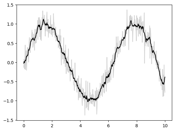
mode 參數控制邊界條件的處理方式;這裡我們使用 mode='same' 以確保輸出與輸入大小相同。
如需更多資訊,請參閱 jax.numpy.convolve() 文件,或與原始 numpy.convolve() 函式相關聯的文件。
基本 N 維卷積#
對於 N 維卷積,jax.scipy.signal.convolve() 提供了類似於 jax.numpy.convolve() 的介面,並推廣到 N 維度。
例如,以下是基於與高斯濾波器卷積來對影像進行去噪的簡單方法
from scipy import datasets
import jax.scipy as jsp

fig, ax = plt.subplots(1, 3, figsize=(12, 5))

# Load a sample image; compute mean() to convert from RGB to grayscale.
image = jnp.array(datasets.face().mean(-1))
ax[0].imshow(image, cmap='binary_r')
ax[0].set_title('original')

# Create a noisy version by adding random Gaussian noise
key = random.key(1701)
noisy_image = image + 50 * random.normal(key, image.shape)
ax[1].imshow(noisy_image, cmap='binary_r')
ax[1].set_title('noisy')

# Smooth the noisy image with a 2D Gaussian smoothing kernel.
x = jnp.linspace(-3, 3, 7)
window = jsp.stats.norm.pdf(x) * jsp.stats.norm.pdf(x[:, None])
smooth_image = jsp.signal.convolve(noisy_image, window, mode='same')
ax[2].imshow(smooth_image, cmap='binary_r')
ax[2].set_title('smoothed');
Downloading file 'face.dat' from 'https://raw.githubusercontent.com/scipy/dataset-face/main/face.dat' to '/home/docs/.cache/scipy-data'.
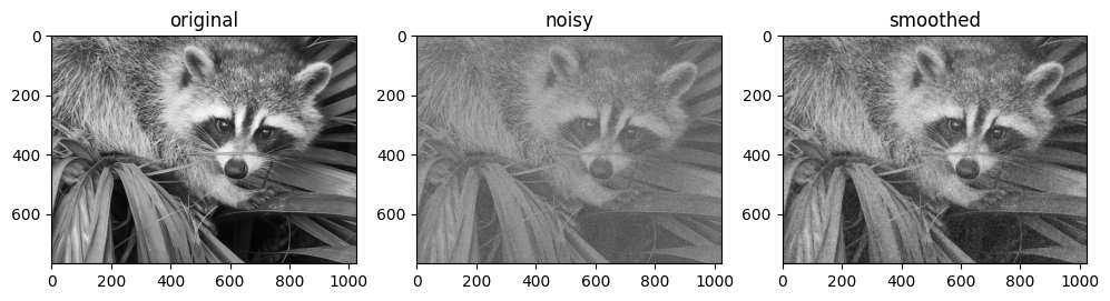
與一維情況一樣,我們使用 mode='same' 來指定我們希望如何處理邊緣。如需 N 維卷積中可用選項的更多資訊,請參閱 jax.scipy.signal.convolve() 文件。
廣義卷積#
對於在建構深度神經網路的背景中通常更有用的更通用類型的批次卷積,JAX 和 XLA 提供了非常通用的 N 維 conv_general_dilated 函式,但如何使用它並不是很明顯。我們將提供一些常見用例的範例。
強烈建議閱讀卷積運算子系列的調查報告,卷積算術指南!
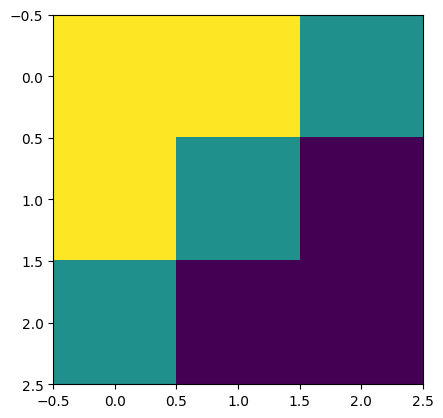
讓我們定義一個簡單的對角邊緣核心
# 2D kernel - HWIO layout
kernel = jnp.zeros((3, 3, 3, 3), dtype=jnp.float32)
kernel += jnp.array([[1, 1, 0],
[1, 0,-1],
[0,-1,-1]])[:, :, jnp.newaxis, jnp.newaxis]
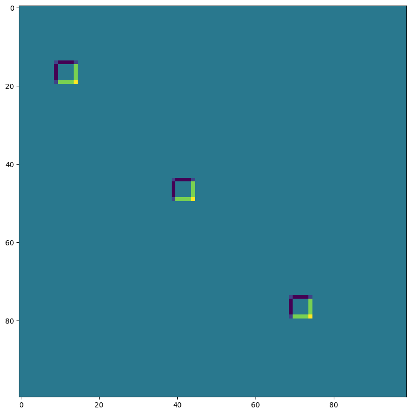
print("Edge Conv kernel:")
plt.imshow(kernel[:, :, 0, 0]);
Edge Conv kernel:
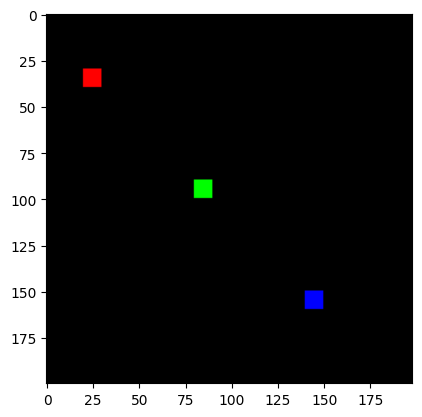
我們將製作一個簡單的合成影像
# NHWC layout
img = jnp.zeros((1, 200, 198, 3), dtype=jnp.float32)
for k in range(3):
x = 30 + 60*k
y = 20 + 60*k
img = img.at[0, x:x+10, y:y+10, k].set(1.0)
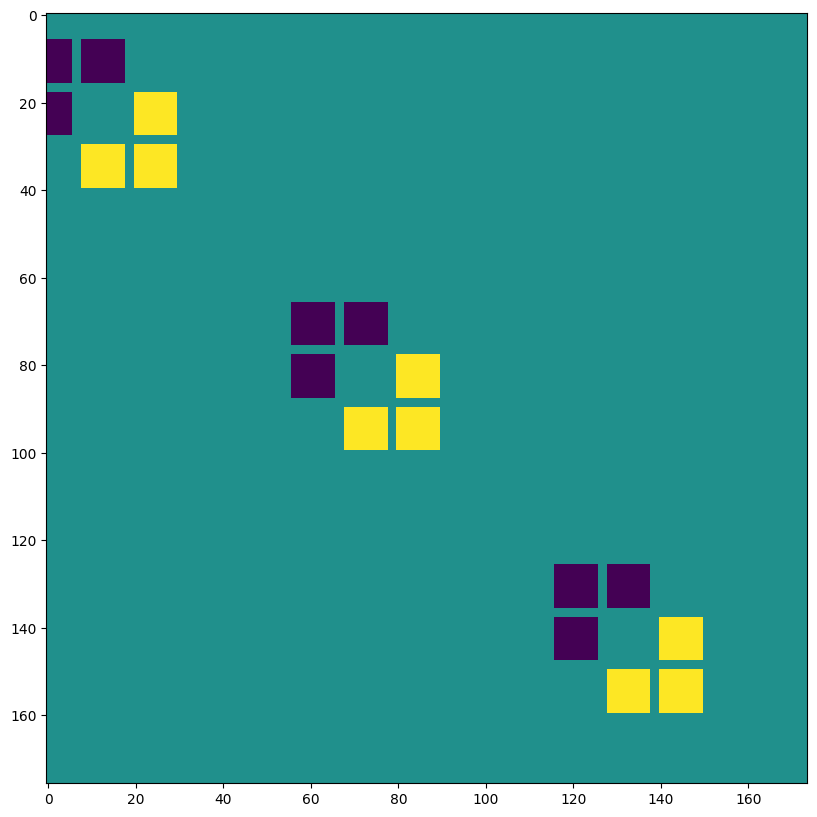
print("Original Image:")
plt.imshow(img[0]);
Original Image:
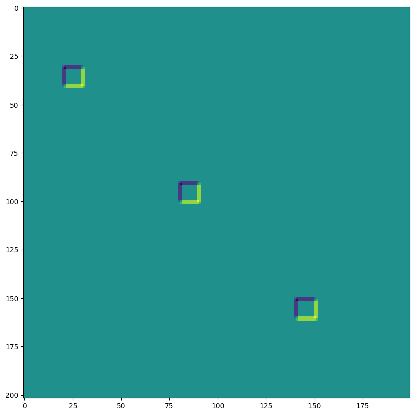
lax.conv 和 lax.conv_with_general_padding#
這些是用於卷積的簡單便利函式
️⚠️ 便利的 lax.conv、lax.conv_with_general_padding 輔助函式假設 NCHW 影像和 OIHW 核心。
from jax import lax
out = lax.conv(jnp.transpose(img,[0,3,1,2]), # lhs = NCHW image tensor
jnp.transpose(kernel,[3,2,0,1]), # rhs = OIHW conv kernel tensor
(1, 1), # window strides
'SAME') # padding mode
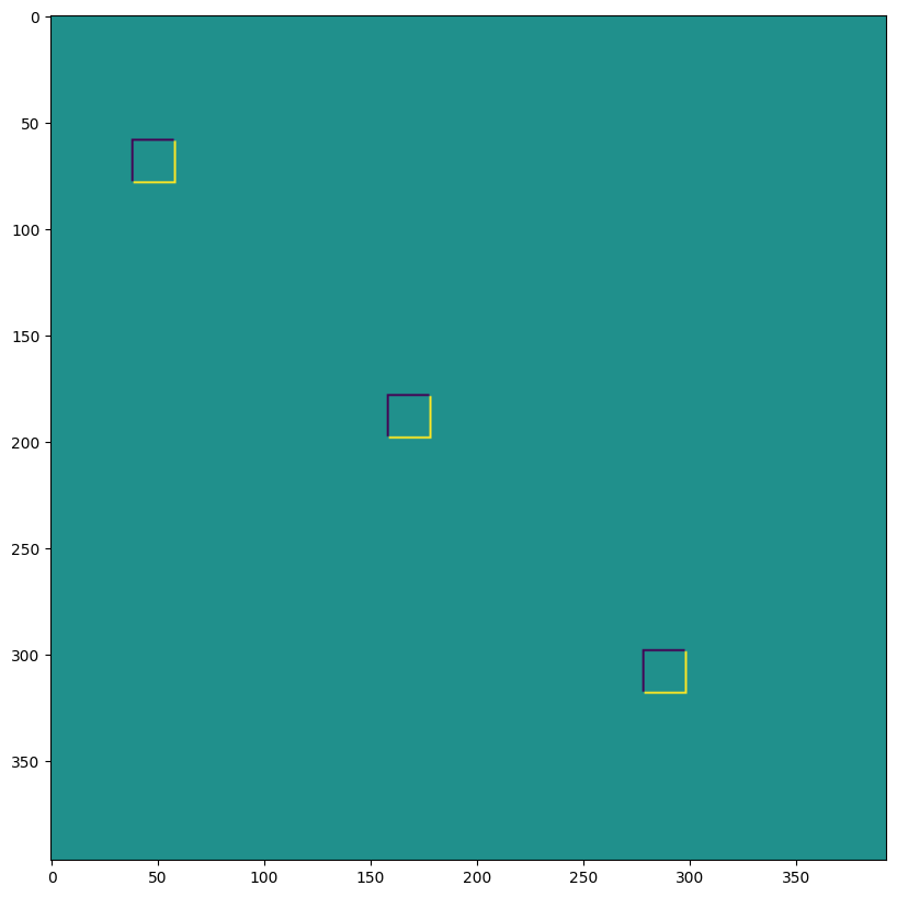
print("out shape: ", out.shape)
print("First output channel:")
plt.figure(figsize=(10,10))
plt.imshow(np.array(out)[0,0,:,:]);
out shape:  (1, 3, 200, 198)
First output channel:

out = lax.conv_with_general_padding(
jnp.transpose(img,[0,3,1,2]), # lhs = NCHW image tensor
jnp.transpose(kernel,[2,3,0,1]), # rhs = IOHW conv kernel tensor
(1, 1), # window strides
((2,2),(2,2)), # general padding 2x2
(1,1), # lhs/image dilation
(1,1)) # rhs/kernel dilation
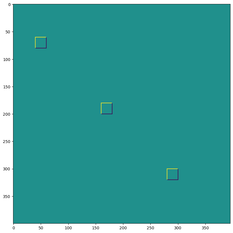
print("out shape: ", out.shape)
print("First output channel:")
plt.figure(figsize=(10,10))
plt.imshow(np.array(out)[0,0,:,:]);
out shape:  (1, 3, 202, 200)
First output channel:
維度編號定義 conv_general_dilated 的維度佈局#
重要的引數是軸佈局引數的 3 元組:(輸入佈局、核心佈局、輸出佈局)
N - 批次維度
H - 空間高度
W - 空間寬度
C - 通道維度
I - 核心輸入通道維度
O - 核心輸出通道維度
⚠️ 為了示範維度編號的彈性,我們為以下的 lax.conv_general_dilated 選擇了 NHWC 影像和 HWIO 核心慣例。
dn = lax.conv_dimension_numbers(img.shape,     # only ndim matters, not shape
                                kernel.shape,  # only ndim matters, not shape
                                ('NHWC', 'HWIO', 'NHWC'))  # the important bit
print(dn)
ConvDimensionNumbers(lhs_spec=(0, 3, 1, 2), rhs_spec=(3, 2, 0, 1), out_spec=(0, 3, 1, 2))
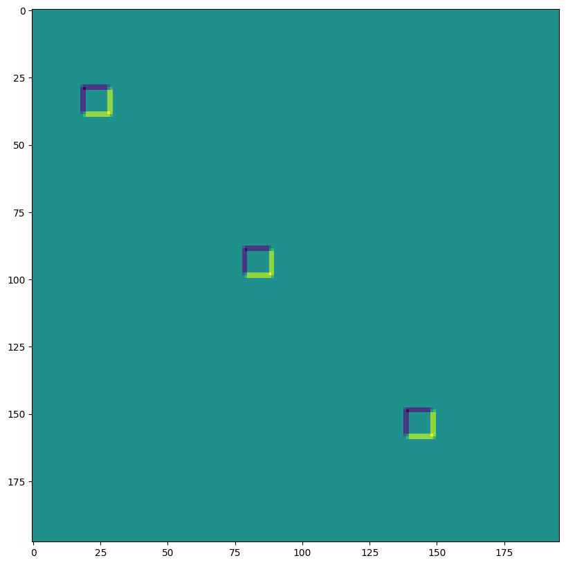
SAME 填充,無步幅,無擴張#
out = lax.conv_general_dilated(img,    # lhs = image tensor
                               kernel, # rhs = conv kernel tensor
                               (1,1),  # window strides
                               'SAME', # padding mode
                               (1,1),  # lhs/image dilation
                               (1,1),  # rhs/kernel dilation
                               dn)     # dimension_numbers = lhs, rhs, out dimension permutation
print("out shape: ", out.shape)
print("First output channel:")
plt.figure(figsize=(10,10))
plt.imshow(np.array(out)[0,:,:,0]);
out shape:  (1, 200, 198, 3)
First output channel:
VALID 填充,無步幅,無擴張#
out = lax.conv_general_dilated(img,     # lhs = image tensor
                               kernel,  # rhs = conv kernel tensor
                               (1,1),   # window strides
                               'VALID', # padding mode
                               (1,1),   # lhs/image dilation
                               (1,1),   # rhs/kernel dilation
                               dn)      # dimension_numbers = lhs, rhs, out dimension permutation
print("out shape: ", out.shape, "DIFFERENT from above!")
print("First output channel:")
plt.figure(figsize=(10,10))
plt.imshow(np.array(out)[0,:,:,0]);
out shape:  (1, 198, 196, 3) DIFFERENT from above!
First output channel:
SAME 填充,2,2 步幅,無擴張#
out = lax.conv_general_dilated(img,    # lhs = image tensor
                               kernel, # rhs = conv kernel tensor
                               (2,2),  # window strides
                               'SAME', # padding mode
                               (1,1),  # lhs/image dilation
                               (1,1),  # rhs/kernel dilation
                               dn)     # dimension_numbers = lhs, rhs, out dimension permutation
print("out shape: ", out.shape, " <-- half the size of above")
plt.figure(figsize=(10,10))
print("First output channel:")
plt.imshow(np.array(out)[0,:,:,0]);
out shape:  (1, 100, 99, 3)  <-- half the size of above
First output channel:
VALID 填充,無步幅,rhs 核心擴張 ~ Atrous 卷積 (過度示範)#
out = lax.conv_general_dilated(img,     # lhs = image tensor
                               kernel,  # rhs = conv kernel tensor
                               (1,1),   # window strides
                               'VALID', # padding mode
                               (1,1),   # lhs/image dilation
                               (12,12), # rhs/kernel dilation
                               dn)      # dimension_numbers = lhs, rhs, out dimension permutation
print("out shape: ", out.shape)
plt.figure(figsize=(10,10))
print("First output channel:")
plt.imshow(np.array(out)[0,:,:,0]);
out shape:  (1, 176, 174, 3)
First output channel:
VALID 填充,無步幅,lhs=輸入擴張 ~ 轉置卷積#
out = lax.conv_general_dilated(img,               # lhs = image tensor
                               kernel,            # rhs = conv kernel tensor
                               (1,1),             # window strides
                               ((0, 0), (0, 0)),  # padding mode
                               (2,2),             # lhs/image dilation
                               (1,1),             # rhs/kernel dilation
                               dn)                # dimension_numbers = lhs, rhs, out dimension permutation
print("out shape: ", out.shape, "<-- larger than original!")
plt.figure(figsize=(10,10))
print("First output channel:")
plt.imshow(np.array(out)[0,:,:,0]);
out shape:  (1, 397, 393, 3) <-- larger than original!
First output channel:
我們可以將最後一個用於例如實作轉置卷積
# The following is equivalent to tensorflow:
# N,H,W,C = img.shape
# out = tf.nn.conv2d_transpose(img, kernel, (N,2*H,2*W,C), (1,2,2,1))

# transposed conv = 180deg kernel rotation plus LHS dilation
# rotate kernel 180deg:
kernel_rot = jnp.rot90(jnp.rot90(kernel, axes=(0,1)), axes=(0,1))
# need a custom output padding:
padding = ((2, 1), (2, 1))
out = lax.conv_general_dilated(img,     # lhs = image tensor
                               kernel_rot,  # rhs = conv kernel tensor
                               (1,1),   # window strides
                               padding, # padding mode
                               (2,2),   # lhs/image dilation
                               (1,1),   # rhs/kernel dilation
                               dn)      # dimension_numbers = lhs, rhs, out dimension permutation
print("out shape: ", out.shape, "<-- transposed_conv")
plt.figure(figsize=(10,10))
print("First output channel:")
plt.imshow(np.array(out)[0,:,:,0]);
out shape:  (1, 400, 396, 3) <-- transposed_conv
First output channel:
1D 卷積#
您不限於 2D 卷積,以下是一個簡單的 1D 示範
# 1D kernel - WIO layout
kernel = jnp.array([[[1, 0, -1], [-1, 0, 1]],
[[1, 1, 1], [-1, -1, -1]]],
dtype=jnp.float32).transpose([2,1,0])
# 1D data - NWC layout
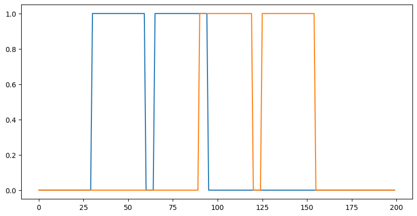
data = np.zeros((1, 200, 2), dtype=jnp.float32)
for i in range(2):
for k in range(2):
x = 35*i + 30 + 60*k
data[0, x:x+30, k] = 1.0
print("in shapes:", data.shape, kernel.shape)
plt.figure(figsize=(10,5))
plt.plot(data[0]);
dn = lax.conv_dimension_numbers(data.shape, kernel.shape,
('NWC', 'WIO', 'NWC'))
print(dn)
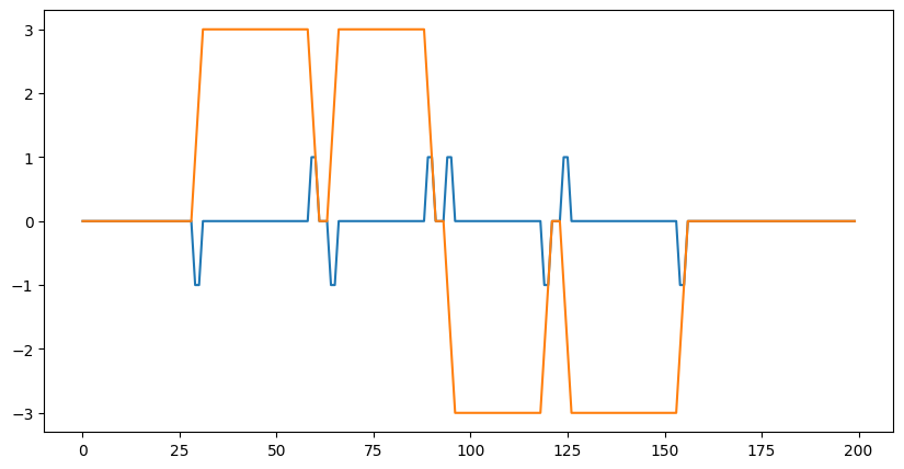
out = lax.conv_general_dilated(data, # lhs = image tensor
kernel, # rhs = conv kernel tensor
(1,), # window strides
'SAME', # padding mode
(1,), # lhs/image dilation
(1,), # rhs/kernel dilation
dn) # dimension_numbers = lhs, rhs, out dimension permutation
print("out shape: ", out.shape)
plt.figure(figsize=(10,5))
plt.plot(out[0]);
in shapes: (1, 200, 2) (3, 2, 2)
ConvDimensionNumbers(lhs_spec=(0, 2, 1), rhs_spec=(2, 1, 0), out_spec=(0, 2, 1))
out shape:  (1, 200, 2)
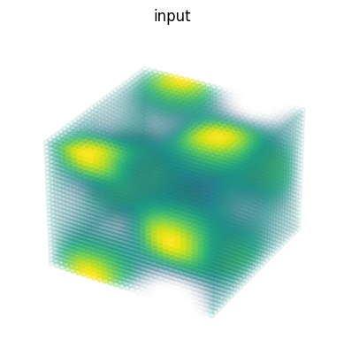
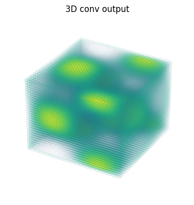
3D 卷積#
import matplotlib as mpl

# Random 3D kernel - HWDIO layout
kernel = jnp.array([
  [[0, 0,  0], [0,  1,  0], [0,  0,   0]],
  [[0, -1, 0], [-1, 0, -1], [0,  -1,  0]],
  [[0, 0,  0], [0,  1,  0], [0,  0,   0]]],
  dtype=jnp.float32)[:, :, :, jnp.newaxis, jnp.newaxis]

# 3D data - NHWDC layout
data = jnp.zeros((1, 30, 30, 30, 1), dtype=jnp.float32)
x, y, z = np.mgrid[0:1:30j, 0:1:30j, 0:1:30j]
data += (jnp.sin(2*x*jnp.pi)*jnp.cos(2*y*jnp.pi)*jnp.cos(2*z*jnp.pi))[None,:,:,:,None]

print("in shapes:", data.shape, kernel.shape)
dn = lax.conv_dimension_numbers(data.shape, kernel.shape,
                                ('NHWDC', 'HWDIO', 'NHWDC'))
print(dn)

out = lax.conv_general_dilated(data,    # lhs = image tensor
                               kernel,  # rhs = conv kernel tensor
                               (1,1,1), # window strides
                               'SAME',  # padding mode
                               (1,1,1), # lhs/image dilation
                               (1,1,1), # rhs/kernel dilation
                               dn)      # dimension_numbers
print("out shape: ", out.shape)

# Make some simple 3d density plots:
def make_alpha(cmap):
  my_cmap = cmap(jnp.arange(cmap.N))
  my_cmap[:,-1] = jnp.linspace(0, 1, cmap.N)**3
  return mpl.colors.ListedColormap(my_cmap)
my_cmap = make_alpha(plt.cm.viridis)
fig = plt.figure()
ax = fig.add_subplot(projection='3d')
ax.scatter(x.ravel(), y.ravel(), z.ravel(), c=data.ravel(), cmap=my_cmap)
ax.axis('off')
ax.set_title('input')
fig = plt.figure()
ax = fig.add_subplot(projection='3d')
ax.scatter(x.ravel(), y.ravel(), z.ravel(), c=out.ravel(), cmap=my_cmap)
ax.axis('off')
ax.set_title('3D conv output');
in shapes: (1, 30, 30, 30, 1) (3, 3, 3, 1, 1)
ConvDimensionNumbers(lhs_spec=(0, 4, 1, 2, 3), rhs_spec=(4, 3, 0, 1, 2), out_spec=(0, 4, 1, 2, 3))
out shape:  (1, 30, 30, 30, 1)